Learned Representations (NLP)
Published on July 07, 2026
Notes from lecture 2 of this NLP series, walking through a generalized CBOW architecture — the “embed → pool → linear classifier” pipeline that underlies how word embeddings are learned.
The diagram in the lecture is a generalized CBOW architecture. It abstracts away the one-hot vectors and focuses on what happens after the embedding lookup.
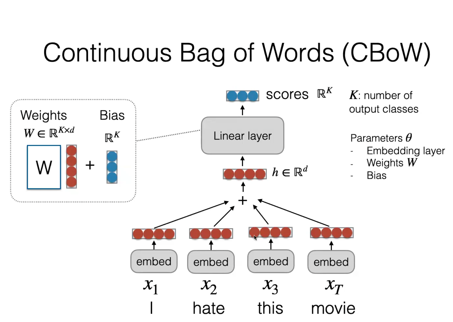
Let’s go through it from bottom to top.
Step 1: Input words
At the bottom are the input words:
x₁      x₂      x₃      ...     x_T
 I     hate    this            movie
Suppose the sentence is “I hate this movie”. Each \(x_i\) is not yet an embedding — it’s simply a token (or equivalently, its vocabulary index).
Step 2: Embedding layer
Each word passes through an embedding lookup:
I        ──embed──> [ 0.2, -0.5,  0.7, ...]
hate     ──embed──> [-0.8,  1.1,  0.4, ...]
this     ──embed──> [ 0.1,  0.0, -0.3, ...]
movie    ──embed──> [ 0.9, -0.4,  0.8, ...]
Each embedding has dimension \(d\), which is why the diagram writes \(h \in \mathbb{R}^d\).
Step 3: Combine the embeddings
The “+” in the diagram is the important part: the embeddings are added together,
\[h = e_1 + e_2 + e_3 + \dots + e_T\]or sometimes averaged,
\[h = \frac{1}{T} \sum_{i=1}^{T} e_i\](The average is more common in Word2Vec CBOW; diagrams often show the sum because it differs only by a constant factor.)
A tiny numeric example:
I        [1, 2, 3]
hate     [2, 4, 6]
this     [3, 1, 0]
movie    [4, 5, 2]

sum     = [10, 12, 11]
average = [2.5, 3, 2.75]
This single vector is the representation of the entire context.
Step 4: Hidden representation
The result is labeled \(h \in \mathbb{R}^d\): the context has now become one dense vector. Everything below the plus sign is essentially
words → embeddings → sum/average → context vector h
Step 5: Linear layer
Next comes a linear layer — just a matrix multiplication plus bias. With \(W \in \mathbb{R}^{K \times d}\) and \(b \in \mathbb{R}^K\),
\[\text{scores} = Wh + b\]Suppose the embedding size is \(d = 100\) and the vocabulary size is \(K = 10{,}000\). Then \(h\) (100 numbers) is multiplied by \(W\) (10,000 × 100) to produce 10,000 scores — one score for every word in the vocabulary.
Step 6: Scores
The output units represent raw scores (logits), for example:
| Word | Score |
|---|---|
| I | -2.1 |
| love | 0.5 |
| movie | 1.9 |
| this | -0.8 |
| great | 4.6 |
| terrible | -1.4 |
A softmax (not shown in the diagram) turns these into probabilities:
\[P(\text{word}) = \text{softmax}(\text{scores})\]The word with the highest probability is the prediction.
Why K output classes?
Because predicting a word is treated as a classification problem. If the vocabulary contains 10,000 words, there are 10,000 possible answers — each output neuron corresponds to one vocabulary word.
What are the parameters?
The trainable parameters are exactly what the diagram lists:
- Embedding matrix. With a vocabulary of 50,000 words and embedding size 300, this is a 50,000 × 300 matrix — each row is the vector for one word.
- Linear layer weights \(W\): 50,000 × 300.
- Bias: one per vocabulary word, so 50,000 numbers.
One subtle point
The example sentence (“I hate this movie”) can be confusing. The diagram illustrates the architecture, not the original Word2Vec CBOW training objective.
In the original Word2Vec CBOW, you remove one word and predict it from its surrounding context:
Sentence:  I hate this movie

Input:   I, this, movie
           ↓ embeddings
           ↓ average
           ↓ linear layer
Predict: hate
Here the target is the missing center word “hate”.
In contrast, the figure is really a generic “embed → pool (sum/average) → linear classifier” pipeline, which is also used for sentence classification tasks. The architecture is almost identical; only the training target changes.
The entire computation in one equation
If the context words have embeddings \(e_1, e_2, \dots, e_T\), the forward pass is:
\[h = \frac{1}{T} \sum_{i=1}^{T} e_i\] \[\text{scores} = Wh + b\] \[P(\text{word} \mid \text{context}) = \text{softmax}(\text{scores})\]Training adjusts both the embedding matrix and the linear layer so that words appearing in similar contexts end up with similar embedding vectors. This is how CBOW learns meaningful word embeddings.
Going deeper: Deep CBOW
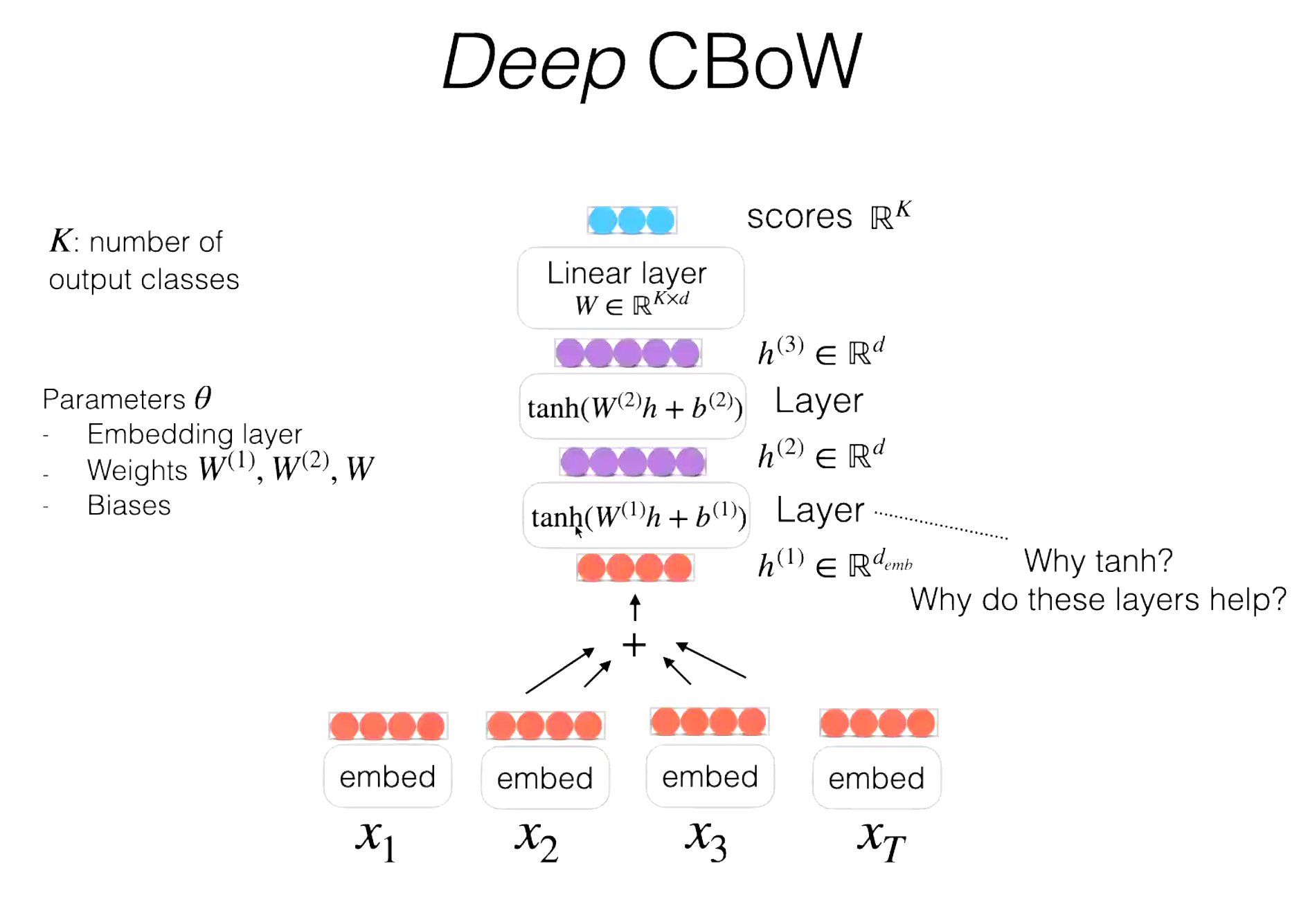
Deep CBOW keeps the same bottom half — embed each word, sum into a context vector \(h^{(1)}\) — but instead of feeding it straight into the output linear layer, it stacks extra hidden layers in between:
\[h^{(2)} = \tanh\!\left(W^{(1)} h^{(1)} + b^{(1)}\right)\] \[h^{(3)} = \tanh\!\left(W^{(2)} h^{(2)} + b^{(2)}\right)\] \[\text{scores} = W h^{(3)} + b\]The addition of \(\tanh\) introduces a non-linearity. This is the whole point: without it, stacking linear layers is useless, because a composition of linear maps collapses into a single linear map — \(W^{(2)}(W^{(1)}h)\) is just another matrix times \(h\). With the non-linearity in between, the extra layers can model combinations of words rather than treating each word’s contribution independently — e.g. “don’t” and “love” appearing together can push the output in a different direction than either word alone.
The parameter list grows accordingly: the embedding layer, the hidden-layer weights \(W^{(1)}, W^{(2)}\) and their biases, and the final output weights \(W\) and bias.
Tags: nlp, embeddings, word2vec, cbow